FlowSOM Clustering#
In this tutorial we are going to review how you can use FlowSOM to cluster single cell cytometry data. To demonstrate the FlowSOM algorithm we will be using the Levine 32 dimensional mass cytometry data originally introduced in the Phenograph paper “Data-Driven Phenotypic Dissection of AML Reveals Progenitor-like Cells that Correlate with Prognosis” in 2015 (https://pubmed.ncbi.nlm.nih.gov/26095251/). You can obtain the Levine data from this GitHub repository: https://github.com/lmweber/benchmark-data-Levine-32-dim/tree/master/data.
import scanpy as sc
import anndata as ann
import numpy as np
import scipy as sp
import pandas as pd
import matplotlib.pyplot as pl
from matplotlib import rcParams
from matplotlib import colors
import seaborn as sb
import datetime
import pytometry as pm


sc.logging.print_versions()
sc.settings.verbosity = 3
-----
anndata     0.9.2
scanpy      1.9.5
-----
PIL                         10.0.1
anyio                       NA
argcomplete                 NA
arrow                       1.3.0
asttokens                   NA
attr                        23.1.0
attrs                       23.1.0
babel                       2.13.0
backcall                    0.2.0
certifi                     2023.07.22
cffi                        1.16.0
charset_normalizer          3.3.0
cloudpickle                 2.2.1
comm                        0.1.4
consensusclustering         NA
cycler                      0.12.0
cython_runtime              NA
dask                        2023.9.3
datashader                  0.15.2
datashape                   0.5.2
dateutil                    2.8.2
debugpy                     1.8.0
decorator                   5.1.1
defusedxml                  0.7.1
entrypoints                 0.4
exceptiongroup              1.1.3
executing                   2.0.0
fastjsonschema              NA
fcsparser                   0.2.7
fqdn                        NA
fsspec                      2023.9.2
h5py                        3.9.0
idna                        3.4
ipykernel                   6.25.2
ipython_genutils            0.2.0
ipywidgets                  8.1.1
isoduration                 NA
jedi                        0.19.1
jinja2                      3.1.2
joblib                      1.3.2
json5                       NA
jsonpointer                 2.4
jsonschema                  4.19.1
jsonschema_specifications   NA
jupyter_events              0.8.0
jupyter_server              2.8.0
jupyterlab_server           2.25.0
kiwisolver                  1.4.5
kneed                       0.8.5
lamin_utils                 0.11.4
llvmlite                    0.41.0
markupsafe                  2.1.3
matplotlib                  3.8.0
minisom                     NA
mpl_toolkits                NA
multipledispatch            0.6.0
natsort                     8.4.0
nbformat                    5.9.2
numba                       0.58.0
numpy                       1.25.2
overrides                   NA
packaging                   23.2
pandas                      1.5.3
param                       1.13.0
parso                       0.8.3
patsy                       0.5.3
pexpect                     4.8.0
pickleshare                 0.7.5
platformdirs                3.11.0
prometheus_client           NA
prompt_toolkit              3.0.39
psutil                      5.9.5
ptyprocess                  0.7.0
pure_eval                   0.2.2
pyct                        0.5.0
pydev_ipython               NA
pydevconsole                NA
pydevd                      2.9.5
pydevd_file_utils           NA
pydevd_plugins              NA
pydevd_tracing              NA
pygments                    2.16.1
pyparsing                   3.1.1
pythonjsonlogger            NA
pytometry                   0.1.4
pytz                        2023.3.post1
readfcs                     1.1.7
referencing                 NA
requests                    2.31.0
rfc3339_validator           0.1.4
rfc3986_validator           0.1.1
rpds                        NA
scipy                       1.11.3
seaborn                     0.12.2
send2trash                  NA
session_info                1.0.0
setuptools                  67.6.0
sitecustomize               NA
six                         1.16.0
sklearn                     1.3.1
sniffio                     1.3.0
sphinxcontrib               NA
stack_data                  0.6.3
statsmodels                 0.14.0
threadpoolctl               3.2.0
tlz                         0.12.0
toolz                       0.12.0
tornado                     6.3.3
tqdm                        4.66.1
traitlets                   5.11.2
typing_extensions           NA
uri_template                NA
urllib3                     2.0.6
wcwidth                     0.2.8
webcolors                   1.13
websocket                   1.6.4
xarray                      2023.9.0
yaml                        6.0.1
zipp                        NA
zmq                         24.0.1
zoneinfo                    NA
-----
IPython             8.16.1
jupyter_client      7.4.9
jupyter_core        5.3.2
jupyterlab          4.0.7
notebook            6.5.6
-----
Python 3.10.12 (main, Jun 11 2023, 05:26:28) [GCC 11.4.0]
Linux-6.2.0-36-generic-x86_64-with-glibc2.35
-----
Session information updated at 2023-11-07 08:47
First we will load the data.
adata = pm.io.read_fcs("./Levine_32dim_notransform.fcs")
adata.var
| n | channel | marker | $PnB | $PnE | $PnR | |
|---|---|---|---|---|---|---|
| Time | 1 | Time | 32 | 0,0 | 1024 | |
| Cell_length | 2 | Cell_length | 32 | 0,0 | 1024 | |
| DNA1 | 3 | DNA1 | 32 | 0,0 | 1024 | |
| DNA2 | 4 | DNA2 | 32 | 0,0 | 1024 | |
| CD45RA | 5 | CD45RA | 32 | 0,0 | 1024 | |
| CD133 | 6 | CD133 | 32 | 0,0 | 1024 | |
| CD19 | 7 | CD19 | 32 | 0,0 | 1024 | |
| CD22 | 8 | CD22 | 32 | 0,0 | 1024 | |
| CD11b | 9 | CD11b | 32 | 0,0 | 1024 | |
| CD4 | 10 | CD4 | 32 | 0,0 | 1024 | |
| CD8 | 11 | CD8 | 32 | 0,0 | 1024 | |
| CD34 | 12 | CD34 | 32 | 0,0 | 1024 | |
| Flt3 | 13 | Flt3 | 32 | 0,0 | 1024 | |
| CD20 | 14 | CD20 | 32 | 0,0 | 1024 | |
| CXCR4 | 15 | CXCR4 | 32 | 0,0 | 1024 | |
| CD235ab | 16 | CD235ab | 32 | 0,0 | 1024 | |
| CD45 | 17 | CD45 | 32 | 0,0 | 1024 | |
| CD123 | 18 | CD123 | 32 | 0,0 | 1024 | |
| CD321 | 19 | CD321 | 32 | 0,0 | 1024 | |
| CD14 | 20 | CD14 | 32 | 0,0 | 1024 | |
| CD33 | 21 | CD33 | 32 | 0,0 | 1024 | |
| CD47 | 22 | CD47 | 32 | 0,0 | 1024 | |
| CD11c | 23 | CD11c | 32 | 0,0 | 1024 | |
| CD7 | 24 | CD7 | 32 | 0,0 | 1024 | |
| CD15 | 25 | CD15 | 32 | 0,0 | 1024 | |
| CD16 | 26 | CD16 | 32 | 0,0 | 1024 | |
| CD44 | 27 | CD44 | 32 | 0,0 | 1024 | |
| CD38 | 28 | CD38 | 32 | 0,0 | 1024 | |
| CD13 | 29 | CD13 | 32 | 0,0 | 1024 | |
| CD3 | 30 | CD3 | 32 | 0,0 | 1024 | |
| CD61 | 31 | CD61 | 32 | 0,0 | 1024 | |
| CD117 | 32 | CD117 | 32 | 0,0 | 1024 | |
| CD49d | 33 | CD49d | 32 | 0,0 | 1024 | |
| HLA-DR | 34 | HLA-DR | 32 | 0,0 | 1024 | |
| CD64 | 35 | CD64 | 32 | 0,0 | 1024 | |
| CD41 | 36 | CD41 | 32 | 0,0 | 1024 | |
| Viability | 37 | Viability | 32 | 0,0 | 1024 | |
| file_number | 38 | file_number | 32 | 0,0 | 1024 | |
| event_number | 39 | event_number | 32 | 0,0 | 1024 | |
| label | 40 | label | 32 | 0,0 | 1024 | |
| individual | 41 | individual | 32 | 0,0 | 1024 |
As you can see, the dataset consists of numerous channels and some meta-variables such as individual and label.
adata[:, "label"].to_df()["label"].value_counts(dropna=False)
NaN     161443
7.0      26366
10.0     21099
8.0      20108
9.0      16520
13.0      6135
2.0       3905
4.0       3295
3.0       2248
11.0      1238
1.0       1207
6.0        916
14.0       513
12.0       330
5.0        304
Name: label, dtype: int64
adata[:, "individual"].to_df()["individual"].value_counts(dropna=False)
1.0    191351
2.0     74276
Name: individual, dtype: int64
channels = [
    "DNA1",
    "DNA2",
    "CD45RA",
    "CD133",
    "CD19",
    "CD22",
    "CD11b",
    "CD4",
    "CD8",
    "CD34",
    "Flt3",
    "CD20",
    "CXCR4",
    "CD235ab",
    "CD45",
    "CD123",
    "CD321",
    "CD14",
    "CD33",
    "CD47",
    "CD11c",
    "CD7",
    "CD15",
    "CD16",
    "CD44",
    "CD38",
    "CD13",
    "CD3",
    "CD61",
    "CD117",
    "CD49d",
    "HLA-DR",
    "CD64",
    "CD41",
]
We want to normalise the channels with a hyperbolic inverse sine with cofactor 5 (as performed in the original paper)
adata_arcsinh = pm.tl.normalize_arcsinh(adata[:, channels], cofactor=5, inplace=False)
We can now cluster our data with the flowsom_clustering function from the tl (tools) module of pytometry. The FlowSOM algorithm works in the following stages:
A self-organising map is trained that learns a low dimensional embedding of the single cell feature space
Consensus clustering (https://github.com/burtonrj/consensusclustering) of the SOM nodes identifies the optimal number of clusters to retain
Each observation is assigned to a cluster according to its nearest meta-cluster in the SOM
The function is going to take as input:
adata- our annotated dataframe of normalised channelskey_added- the key to add the cluster labels undersom_dim- the size of the self-organising map; (10, 10) is the default size used by the original FlowSOM implementation and usually does not need to be alteredsigma- this controls the radius of the neighbourhood function and again the default value of 1.0 works well in most caseslearning_rate- controls the size of weight vector in learning of SOM and the default value of 0.5 works well in most casesbatch_size- adjust if you have memory constraintsseed- random seed for reproducibilitymin_clusters- the minimum number of clusters when searching for the optimal number of clusters in consensus clusteringmax_clusters- the maximum number of clusters when searching for the optimal number of clusters in consensus clusteringreturn_clustering_objs- if True, the SOM and Consensus Clustering objects are returned; this can be helpful for inspecting the results as shown laterverbose- show progress bars etccopy- copy theadataobject (recommended)agglomerative_clustering_kwargs- keyword arguments passed to theAgglomerativeClusteringScikit-Learn object used by the consensus clustering
adata_flowsom, cluster_objs = pm.tl.flowsom_clustering(
    adata=adata_arcsinh,
    key_added="flowsom_clusters",
    som_dim=(10, 10),
    sigma=1.0,
    learning_rate=0.5,
    batch_size=500,
    seed=42,
    min_clusters=10,
    max_clusters=20,
    return_clustering_objs=True,
    verbose=True,
    inplace=True,
    agglomerative_clustering_kwargs={"metric": "euclidean", "linkage": "ward"},
)
 [ 500 / 500 ] 100% - 0:00:00 left
 quantization error: 3.422194930315085
adata_flowsom.obs["flowsom_clusters"].value_counts()
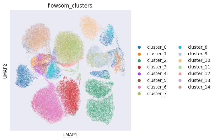
cluster_6     50159
cluster_7     41397
cluster_2     34354
cluster_3     31562
cluster_0     23688
cluster_10    19259
cluster_14    17600
cluster_8     10731
cluster_9     10146
cluster_1      9226
cluster_4      6871
cluster_12     4179
cluster_11     3970
cluster_5      1406
cluster_13     1079
Name: flowsom_clusters, dtype: int64
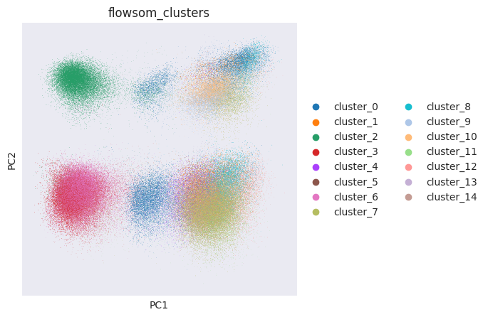
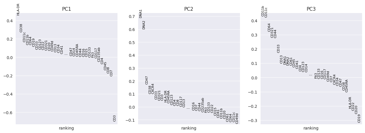
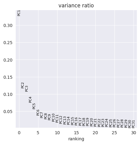
FlowSOM has generated 15 clusters. Lets visualise them using PCA and UMAP:
sc.pp.pca(adata_flowsom)
pl.rcParams["figure.figsize"] = (5, 5)
sc.pl.pca_overview(
    adata_flowsom,
    color="flowsom_clusters",
)
computing PCA
    with n_comps=33
    finished (0:00:00)
/home/ross/Projects/pytometry/venv/lib/python3.10/site-packages/scanpy/plotting/_tools/scatterplots.py:391: UserWarning: No data for colormapping provided via 'c'. Parameters 'cmap' will be ignored
  cax = scatter(
sc.pp.pca(adata_flowsom, n_comps=10)
sc.pp.neighbors(adata_flowsom, n_neighbors=15, use_rep="X_pca")
computing PCA
    with n_comps=10
    finished (0:00:00)
computing neighbors
/home/ross/Projects/pytometry/venv/lib/python3.10/site-packages/numba/np/ufunc/parallel.py:371: NumbaWarning: The TBB threading layer requires TBB version 2021 update 6 or later i.e., TBB_INTERFACE_VERSION >= 12060. Found TBB_INTERFACE_VERSION = 12050. The TBB threading layer is disabled.
  warnings.warn(problem)
    finished: added to `.uns['neighbors']`
    `.obsp['distances']`, distances for each pair of neighbors
    `.obsp['connectivities']`, weighted adjacency matrix (0:00:23)
sc.tl.umap(adata_flowsom)
computing UMAP
    finished: added
    'X_umap', UMAP coordinates (adata.obsm) (0:01:50)
sc.pl.umap(adata_flowsom, color="flowsom_clusters")
/home/ross/Projects/pytometry/venv/lib/python3.10/site-packages/scanpy/plotting/_tools/scatterplots.py:391: UserWarning: No data for colormapping provided via 'c'. Parameters 'cmap' will be ignored
  cax = scatter(
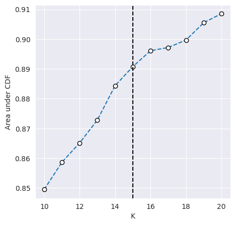
We can inspect why 15 clusters were chosen by accessing the ConsensusClustering object returned by the our FlowSOM function. Consensus clustering works by calculating the consensus matrix of observations across random resamples of our data - stable clustering should result in observations consistently existing within the same or different clusters, if they sometimes appear in the same cluster or sometime do not, this suggests the clustering is unstable.
We can plot the CDF of the consensus matrix across different k clusters and observe the change point at which the area under the CDF no longer increased with the same magnitude. The plots below show the change point as detected by consensus clustering (first plot) and the CDF for each value of k (second plot).
cluster_objs["consensus_clustering"].plot_auc_cdf()
<Axes: xlabel='K', ylabel='Area under CDF'>
cluster_objs["consensus_clustering"].plot_cdf()
<Axes: xlabel='Consensus index value', ylabel='CDF'>
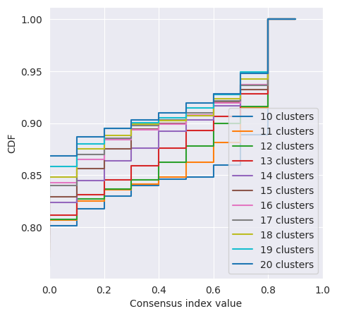
The change in CDF below and above a k of 15 is subtle and we would expect ideal clustering to have consensus index values occuring around 0 or 1, but biological data is often noisy and consensus clusters can be difficult to identify.
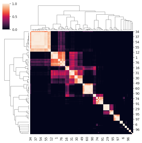
The consensus matrix for the chosen k of 15 is shown below. Notice how for many observations a clear consensus is established along the diagonal but some observations are more difficult and have a ‘fuzzy’ allocation across clusters.
cluster_objs["consensus_clustering"].plot_clustermap(15, figsize=(6, 6))
/home/ross/Projects/pytometry/venv/lib/python3.10/site-packages/seaborn/matrix.py:560: UserWarning: Clustering large matrix with scipy. Installing `fastcluster` may give better performance.
  warnings.warn(msg)
/home/ross/Projects/pytometry/venv/lib/python3.10/site-packages/seaborn/matrix.py:560: UserWarning: Clustering large matrix with scipy. Installing `fastcluster` may give better performance.
  warnings.warn(msg)
<seaborn.matrix.ClusterGrid at 0x7f50b5846740>
