Quickstart#
import pytometry as pm
import readfcs
import anndata
from matplotlib import rcParams
/home/runner/work/pytometry/pytometry/.nox/build-3-9/lib/python3.9/site-packages/tqdm/auto.py:21: TqdmWarning: IProgress not found. Please update jupyter and ipywidgets. See https://ipywidgets.readthedocs.io/en/stable/user_install.html
  from .autonotebook import tqdm as notebook_tqdm
Read fcs file example from the readfcs package. The fcs file was part of the following reference and originally deposited on the FlowRepository.
path_data = readfcs.datasets.Oetjen18_t1()
adata = pm.io.read_fcs(path_data)
assert isinstance(adata, anndata._core.anndata.AnnData)
Next, we split the data matrix into the marker intensity part and the FSC/SSC part. Moreover, we move all height related features to the .obs part of the anndata file. Notably. the function split_signal checks if a feature name is either FSC/SSC or whether a name endswith -A for area related features and -H for height related features.
pm.pp.split_signal(adata, var_key="channel")
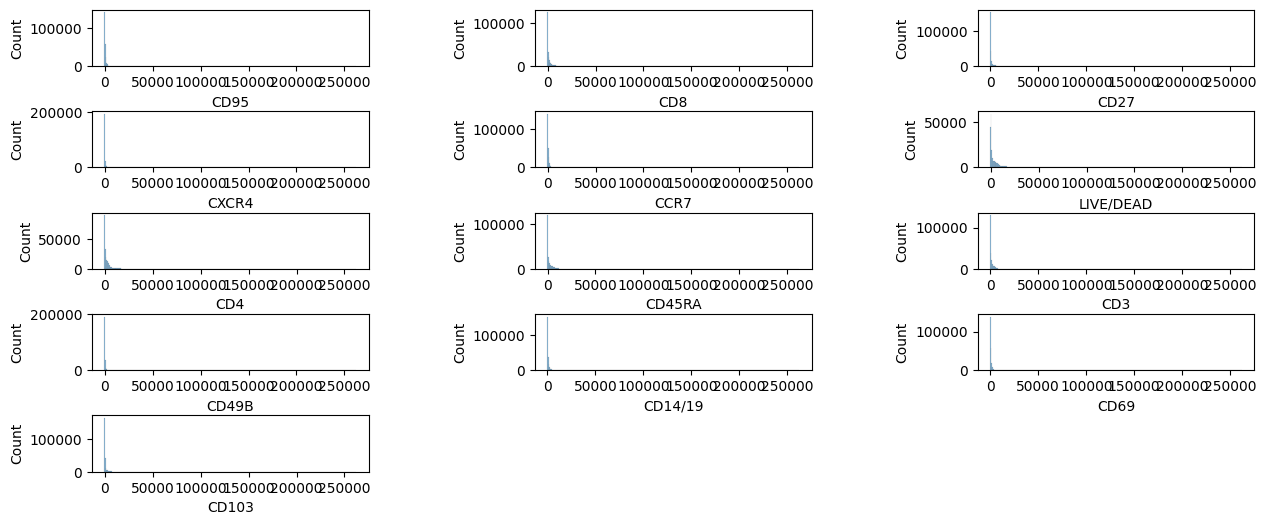
We can plot the fluorescent marker intensity distribution with the plotdata function.
pm.pl.plotdata(adata)
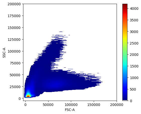
For 2D distribution plots, we use the scatter_density function.
rcParams["figure.figsize"] = (6, 5)
pm.pl.scatter_density(adata, x_lim=[-5e3, 2e5], y_lim=[-5e3, 2e5])
Compensate with the compensation matrix that is deposited in the FCS file. The compensate function also accepts a custom compensation matrix.
pm.pp.compensate(adata)
For normalization, pytometry provides several different approaches:
adata_arcsinh = pm.tl.normalize_arcsinh(adata, cofactor=150, inplace=False)
adata_biexp = pm.tl.normalize_biExp(adata, inplace=False)
adata_logicle = pm.tl.normalize_logicle(adata, inplace=False)
adata_autologicle = pm.tl.normalize_autologicle(adata, inplace=False)
Save data to HDF5 file format.
adata.write("example.h5ad")